Professional Portfolio Optimization Spreadsheet Calculator
Price
USD69.00 - Purchase (For a limited time, get it free at the bottom of this page.)
License
Commercial License
System Requirements
Microsoft® Windows 7, Windows 8 or Windows 10
Windows Server 2003, 2008, 2012 or 2016
512 MB RAM
5 MB of Hard Disk space
Excel 2007, 2010, 2013 or 2016
Portfolio Optimization Spreadsheet
Background
In 1952, Harry Markowitz published a paper on portfolio selection and the effects of diversification on security returns. His works have a great impact on modern finance and have led to the development of the Capital Asset Pricing Model by William Sharpe, Linter and Mossin.In the Portfolio Risk spreadsheet, we have developed a model to calculate the Returns, Mean, Variance and Standard Deviation of a Portfolio based on historical prices. The calculation allows us to see the effects of diversification in the Portfolio. We are taking a step further in this Portfolio Optimization spreadsheet by optimizing the allocation of the assets in the portfolio using Markowitz theory.
We will start with a worksheet that models the Risk Reward Trade Off Line followed by by a worksheet that models Portfolio Optimization of 2 Assets. With these two worksheets as a basis, we will use the Microsoft Excel Solver to model the complex Portfolio Optimization of more than 2 assets. Finally we will integrate our portfolio optimization model with stock prices downloaded from https://finance.yahoo.com. A regression of the historical prices will be performed automatically and the output average returns, correlations, variances and covariances will be used for the portfolio optimization model.
Risk Reward Trade Off Line
The basic principle of the Risk Reward Trade Off Line is the more risk you take, the higher your reward. Of course, the flip side is the possibility of you losing more money. Markowitz theory allows us to vary the amount of risk we undertake in the hope of achieving the returns we expected. The basic concept is to build a portfolio which consists of a normal asset like a stock or a bond with another Riskless Asset like the U.S Treasury Bills. By varying the proportion of each asset, it allows us to vary the amount of risk we wish to undertake vs the returns we hope to achieve.Risk Reward Trade Off Line Spreadsheet
The model in the "PortfolioRiskRewardTradeOffLine" worksheet allows us to combine the normal asset and a Riskless asset to model the Risk Reward Trade Off Line.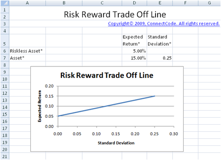
Inputs
- Expected Return Riskless Asset - This can be the published rate of a U.S Treasury Bill or an assumed riskless rate.
- Standard Deviation of Riskless Asset - This is assumed to be zero as the asset is considered riskless.
- Expected Return of Asset - This can be estimated by using historical prices of the asset or an assumed expected return.
- Standard Deviation of Asset - This can be estimated by calculating the standard deviation of the asset from historical prices and assumed standard deviation.
Outputs
The worksheet uses the Portfolio theory to calculate the expected return of the portfolio using the following formula:Expected Return of Portfolio = Weight of normal asset * Expected Return of normal asset + Weight of Riskless asset + Expected Return of Riskless asset.
The standard deviation of the portfolio is the proportion of total assets invested in the risky asset multiply by the standard deviation of the risky asset. This is because the standard deviation of the riskless asset is considered to be zero.
Risk Reward Trade Off Line
The graph shows the different proportion of the normal and Riskless asset. It is simple to see that by investing proportionately more on the normal asset, it may allow us to achieve more returns but at the same time will subject us to more risks. Thus the risk appetite of the investor will determine the various proportions of the portfolio to use.
Correlations of Assets
One of the basic aspects of building a portfolio is to include assets which are negatively or have a small positive correlation with each other. When the assets in a portfolio do not move in the same direction, it is thought to be safer as they do not fluctuate as much. In the next few sections, we will see correlation between the different assets to be an assumed number or calculated from the regression of historical asset prices.Portfolio Optimization (2 Assets)
In the "PortfolioOptimization2Assets" worksheet, we will use Markowitz theory to optimize the proportions of the 2 normal risky assets and the riskless asset in the portfolio. By optimizing the portfolio, we will have a portfolio that is considered as an efficient portfolio.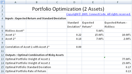
Efficient Portfolio
A efficient portfolio is one that combines the different assets to provide the highest level of expected return while undertaking the lowest level of risk.Efficient Frontier
The graph below shows the attainable set of portfolios by combining the different risky assets as dark dots. From the point X to the point Y in the blue curve, it allows us to achieve highest level of return with the minimal risk we have to undertake. This set of portfolios is known as the efficient frontier. The efficient frontier has been proven to be a hyperbola curve when expected return is plotted against standard deviation.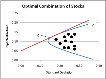
Tangency Portfolio
The Tangency Portfolio is a portfolio that is on the efficient frontier with the highest return minus risk free rate over risk. In other words, it is the portfolio with the highest Sharpe ratio.Inputs
- Expected Return of Riskless Asset - This can be determined from the U.S Treasury Bills or Bonds. The standard deviation of the Riskless asset is not required as this asset is considered riskless.
- Expected Return of Asset 1 - This can be estimated by using historical prices of the asset.
- Expected Return of Asset 2 - This can be estimated by using historical prices of the asset.
- Standard Deviation of Asset 1 - This can be estimated by calculating the standard deviation of the asset from historical prices.
- Standard Deviation of Asset 2 - This can be estimated by calculating the standard deviation of the asset from historical prices.
- Correlation of Asset 1 with Asset 2 - You can use the AssetsCorrelations spreadsheet to determine the correlation of the two assets using historical prices. Or enter an assumed correlation between the two assets.
Outputs
The following four fields are the most important output of this worksheet model. They are the weights of the two different assets that give us the optimal portfolio based on Markowitz theory. The Standard Deviation and the expected Rate of Return are also calculated.- Optimal Portfolio Weight of Asset 1
- Optimal Portfolio Weight of Asset 2
- Optimal Portfolio Standard Deviation
- Optimal Portfolio Rate of Return
Usage of Optimal Portfolio
This section of the worksheet allows you to enter the amount to invest and it will use the Optimal Portfolio weights to calculate the amount to invest in the Riskless Asset, Asset 1 and Asset 2. By entering the Expected Rate of Return, it uses the Risk Reward Trade Off Line to vary the proportion of the Portfolio of normal assets and Riskless Asset.
Optimal Combination of Risky Assets Curve
The optimal combination of risky assets curve is plotted using the following fields by varying the weights in Asset 1 and 2 and calculating the Standard Deviation and Expected Return.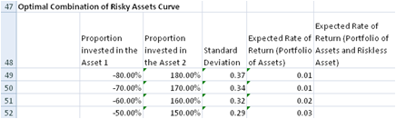
- Proportion invested in the Asset 1 - This field contains the varying weights of Asset 1.
- Proportion invested in the Asset 2 - This field contains the varying weights of Asset 2.
- Standard Deviation - Standard Deviation of the portfolio with the varying weights of Asset 1 and 2.
- Expected Rate of Return (Portfolio of Assets) - Expected Rate of Return of the portfolio with the varying weights of Asset 1 and 2.
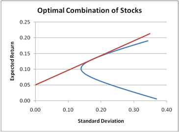
Efficient Trade Off Line
The Efficient Trade Off Line shows the different proportion of the normal and Riskless assets. The following field is added to the curve in the previous section.- Expected Rate of Return (Portfolio of Assets and Riskless Asset)
Portfolio Optimization (7 Assets)
In the "Portfolio Optimization (2 Assets)" worksheet, the formulas for calculating the Expected Return, Standard Deviation and Optimal Portfolio is entered directly into the different cells of the spreadsheet. As the number of assets increase, the worksheet becomes more complex. The correlations, variances and covariances between the different assets will need to be calculated. The optimal portfolio calculation also becomes more complicated with the addition of more variables. In this worksheet, a portfolio of 7 assets are optimized using Markowitz theory. The complex formulas are calculated using Matrix equations and the optimal portfolio is determined using the Solver in Microsoft Excel. With this worksheet, you will be able to customize a portfolio optimization model for any number of assets quickly and easily.Setup Microsoft Excel Solver
In general, the Solver is used for solving optimization problems. In our case, the Solver is used for finding the weights of the assets in the portfolio that maximizes returns while minimizing risks. It is important that the Solver option is enabled in your Excel. Follow the steps below to make sure Solver is ready for use.1. Click the Microsoft Office Button
2. Click on the Excel Options Button
3. Click on Add-Ins, and then in the Manage box, select Excel Add-ins.
4. Click on the Go Button.
5. In the Add-Ins available box, select the Solver Add-in check box, and then click OK. If you are prompted that Solver is not installed, click on Yes to install is.
The Solver Add-In is available in the Analysis group on the Data tab. Try to read the Help on Solver and play around with the examples provided.
Using Microsoft Excel Solver in this spreadsheet model
In most portfolio optimization models, the Solver is required to be use in incremental steps to plot the Optimal Portfolio Curve. This makes the model difficult to use as you are required to perform many steps to arrive with the optimal portfolio. The issue is overcome in this model by using Visual Basic Applications (VBA) code to automate the steps to use the Solver. The source code of the VBA to automate the calculations is explained later in one of the sections. Basically, with a one click of a button the optimal portfolio can be determined.Inputs
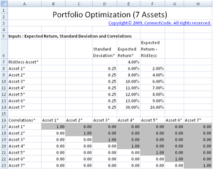
As in the "PortfolioOptimization2Assets" worksheet, this worksheet requires the Standard Deviation and Expected Return of the Riskless and normal risky assets as inputs. The correlations between the different assets are also required. The grey out portion in the spreadsheet above does not require any inputs as their values are a mirror of the portion in light color in the table.
After keying in the inputs as above, the following actions are available. To calculate the optimal portfolio weights and plot the optimal portfolio curve, click on the "Plot Optimal Portfolio Curve" button. To simply calculate the optimal portfolio weights, click on the "Calculate Optimal Portfolio" button.
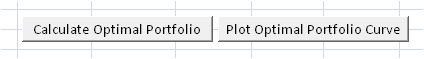
- Calculate Optimal Portfolio - This will call the CalculateOptimalPortfolio macro. We will describe this macro in details later.
- Plot Optimal Portfolio Curve - This will call the SolveEfficientFrontier macro. We will describe this macro in details laster.
Outputs
Covariances The Covariances of the assets are used in the calculation of the optimal portfolio. It is calculated using the formula below:Covariances of Asset X with Asset Y = Standard Deviation of Asset X * Standard Deviation of Asset Y * Correlation of Asset X with Asset Y

Outputs : Optimal Portfolio and Usage of Optimal Portfolio
The Optimal Portfolio section refers to the fields from the Optimal Portfolio Working cells. Both the fields in the Optimal Portfolio and Usage of Optimal Portfolio sections are quite similar to the fields in the "Portfolio Optimization (2 Assets)" worksheet, thus we will not be going into details here.
Optimal Portfolio Working Cells
The cells in this section of the worksheet are used by Solver for performing optimization to determine the Optimal Portfolio weights. The following fields are used in different ways during the optimization process. The optimization processes include the determination of the Minimum Variance Portfolio, the Optimal Portfolio Curve and the Tangency Portfolio.
- Tangency Slope
- Optimal Portfolio Variance
- Optimal Portfolio Standard Deviation
- Weight in Asset 1
- Weight in Asset 2
- Weight in Asset 3
- Weight in Asset 4
- Weight in Asset 5
- Weight in Asset 6
- Weight in Asset 7
- Sum - Sum of all the weights.
The Minimum Variance Portfolio is a portfolio where the weights of the different assets results in a portfolio with the minimum standard deviation. When the button "Plot Optimal Portfolio Curve" buttons as described in section 1.6.3 is clicked on, the minimum Variance Portfolio will be determined using Microsoft Excel Solver as one of the steps to plot the curve. The model will use the Solver internally to determine the weights of the different assets required to have a portfolio with the minimum standard deviation. The following fields are automatically changed by Solver.
- Weight in Asset 1
- Weight in Asset 2
- Weight in Asset 3
- Weight in Asset 4
- Weight in Asset 5
- Weight in Asset 6
- Weight in Asset 7
Determine the Optimal Portfolio Curve
To plot the Optimal Portfolio Curve, we can perform the following steps:
1. Use the standard deviation of the Minimum Variance Portfolio.
2. Find the maximum and minimum Expected Return of the Portfolio.
3. Plot the graph as shown below.
4. Repeat the above steps by increasing the standard deviation of the Minimum Variance Portfolio by a certain percent.

The table below shows the percentage of the standard deviation increased by the model when repeating the steps above.
| X-Axis (Standard Deviation) | Y-Axis (Expected Return) | Comments |
| Optimal Portfolio Standard Deviation | Find both the minimum and maximum Expected Return | |
| Optimal Portfolio Standard Deviation + 5% | Find both the minimum and maximum Expected Return | First vertical line on the graph above. |
| Optimal Portfolio Standard Deviation + 10% | Find both the minimum and maximum Expected Return | Second vertical line on the graph above. |
| Optimal Portfolio Standard Deviation + 50% | Find both the minimum and maximum Expected Return | Third vertical line on the graph above. |
| Optimal Portfolio Standard Deviation + 80% | Find both the minimum and maximum Expected Return | Fourth vertical line on the graph above. |
The Sum field is also used as a constraint for Microsoft Excel Solver. During the process for optimization, the sum of the weights from Solver must satisfy the constraint of 1.
Determine the Tangency Portfolio
The "Tangency Slope" is defined as follows:
Tangency Slope = (Return - Riskless Rate) / Standard Deviation
This is also known as the Sharpe Ratio. Thus the Solver is trying to determine the weights of a portfolio with the maximum Sharpe Ratio.
Internally, the model uses the Solver to determine the maximum value of "Tangency Slope" by varying the following:
- Weight in Asset 1
- Weight in Asset 2
- Weight in Asset 3
- Weight in Asset 4
- Weight in Asset 5
- Weight in Asset 6
- Weight in Asset 7
Automating Solver
The numerous steps to be carried out above using Solver will be tedious if we are to perform it manually. This portfolio optimization model includes a Visual Basic for Applications program to automate the steps. The details will be useful if you are thinking of customizing the model. The information will not be required if you are just using the model.
CalculateOptimalPortfolio VBA Macro
This macro is called when the "Calculate Optimal Portfolio" button from the Inputs section is clicked. The macro is explained using VBA Code comments as highlighted in blue below.
Sub CalculateOptimalPortfolio()

SolverReset
'Reset the Solver
SolverOk SetCell:="$C$92", MaxMinVal:=1,
         ValueOf:="0", ByChange:="$I$95:$O$95"
SolverAdd CellRef:="$P$95", Relation:=2, FormulaText:="1"
'Request the Solver to find the maximum value of the
'Tangency Portfolio in cell $C$92
'by changing the weights in $I$95 to $O$95
'The constraint for the Solver when finding the optimal weights
'is such that the total
'value of the weights must be equal to 1.
SolverOk SetCell:="$C$92", MaxMinVal:=1, ValueOf:="0",
         ByChange:="$I$95:$O$95"
SolverOptions MaxTime:=100, Iterations:=100, Precision:=0.000001,
              AssumeLinear :=False, StepThru:=False,
              Estimates:=1, Derivatives:=1, SearchOption:=1,
              IntTolerance:=5, Scaling:=False,
              Convergence:=0.0001, AssumeNonNeg:=True
'Request the Solver to find the maximum value of
'the Tangency Portfolio in cell $C$92
'by changing the weights in $I$95 to $O$95
'The weights cannot have negative values.
SolverOk SetCell:="$C$92", MaxMinVal:=1, ValueOf:="0",
         ByChange:="$I$95:$O$95"
SolverSolve UserFinish:=True
SolverFinish KeepFinal:=1
Range("A46").Select

End Sub
SolveEfficientFrontier VBA Macro
This macro is called when the "Plot Optimal Portfolio Curve" button from the Inputs section is clicked. In summary, the steps performed are described previously. The steps are shown again below:
1. Use the standard deviation of the Minimum Variance Portfolio. 2. Find the maximum and minimum Expected Return of the Portfolio. 3. Plot the graph as shown below. 4. Repeat the above steps by increasing the standard deviation of the Minimum Variance Portfolio by a certain percent.
The macro is explained in details using VBA Code comments as highlighted in blue below.
    SolverReset
    SolverOk SetCell:="$D$95", MaxMinVal:=2, ValueOf:="0",
             ByChange:="$I$95:$O$95"
    SolverAdd CellRef:="$P$95", Relation:=2, FormulaText:="1"
    SolverOk SetCell:="$D$95", MaxMinVal:=2, ValueOf:="0",
             ByChange:="$I$95:$O$95"
    SolverOptions MaxTime:=100, Iterations:=100,
		Precision:=0.000001,
                  AssumeLinear :=False, StepThru:=False,
                  Estimates:=1, Derivatives:=1,
		SearchOption:=1,
                  IntTolerance:=5, Scaling:=False,
                  Convergence:=0.0001, AssumeNonNeg:=True
    SolverOk SetCell:="$D$95", MaxMinVal:=2,
             ValueOf:="0", ByChange:="$I$95:$O$95"
    SolverSolve UserFinish:=True
    SolverFinish KeepFinal:=1
                    'Find the weights of the different assets in the portfolio
   'that gives the minimum standard
   'deviation
    Range("C95:P95").Select
    Selection.Copy
    Range("C98").Select
    Selection.PasteSpecial Paste:=xlPasteValues,
			   Operation:=xlNone,
                               SkipBlanks :=False,
			   Transpose:=False
                    'Copy the output to row 98
    minSD = Range("$D$98").Value
    minSD = minSD * 1.05
                    'Increase the value of the standard deviation by 5%
    SolverReset
    SolverOk SetCell:="$E$95", MaxMinVal:=1,
             ValueOf:="0", ByChange:="$I$95:$O$95"
    SolverAdd CellRef:="$P$95", Relation:=2,
		  FormulaText:="1"
    SolverOk SetCell:="$E$95", MaxMinVal:=1,
             ValueOf:="0", ByChange:="$I$95:$O$95"
    SolverAdd CellRef:="$D$95", Relation:=2,
		  FormulaText:=minSD
    SolverOk SetCell:="$E$95", MaxMinVal:=1,
             ValueOf:="0", ByChange:="$I$95:$O$95"
    SolverOptions MaxTime:=100, Iterations:=100,
			Precision:=0.000001,
                	AssumeLinear :=False, StepThru:=False,
			Estimates:=1,
                  Derivatives:=1, SearchOption:=1,
			IntTolerance:=5,
                  Scaling:=False, Convergence:=0.0001,
                  AssumeNonNeg:=True
    SolverOk SetCell:="$E$95", MaxMinVal:=1, ValueOf:="0",
                  ByChange:="$I$95:$O$95"
    SolverSolve UserFinish:=True
    SolverFinish KeepFinal:=1
                    'Find a portfolio that satisfies
    'the new standard deviation.
    'Basically, the expected return values
    'will be plotted in the graph.
    Range("C95:P95").Select
    Selection.Copy
    Range("C99").Select
    Selection.PasteSpecial Paste:=xlPasteValues,
			   Operation:=xlNone,
                               SkipBlanks :=False,
			   Transpose:=False
    'Copy the output to row 99

    'Repeat the above steps to plot the Optimal Portfolio Curve
    .
    .
    .
Portfolio Optimization (7 Assets) by performing regression on historical prices
The "AutomaticPortfolioOptimization.xls" spreadsheet reuses the "PortfolioOptimization7Assets" worksheet in the "PortfolioOptimization.xls" spreadsheet. Basically the spreadsheet downloads the stock price of the 7 seven assets specified, automatically calculates the average returns, standard deviation, correlation, variances and covariances.PortInternal Worksheet
This worksheet is used internally by the calculator. The columns contain data that include Date, Open, High, Low, Close, Volume and Adj Close.The Returns column is calculated by the VBA macro which is described below. It uses the latest Adj Close and the previous Adj Close to calculate the periodic rate of return. The formula used is shown below:
Returns = (Latest Adj Close - Previous Adj Close) / Previous Adj Close
The Returns column is tabulated for use in the calculation of the Correlation, Covariance and Variance output.
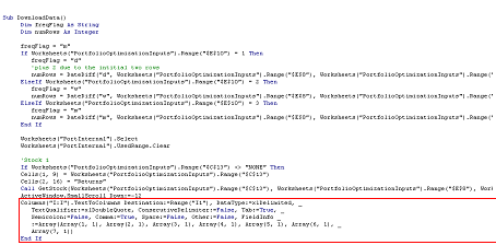
How is the data downloaded?
The Excel spreadsheet uses the macro DownloadData to automatically populate the data in the 'PortInternal' worksheet. If you goto Developer->Visual Basic and open up the Microsoft Visual Basic Editor. After that, double click on the 'VBA Project (AutomaticPortfolioOptimization.xls)' and open up Module->Module1. This module contains all the source code for automatically downloading the data.GetStock subroutine
The VBA code for the GetStock subroutine is listed below. This function downloads data from https://finance.yahoo.com by specifying a Stock Symbol, Start Date and End Date. The last "desti" parameter specifies the location to place the downloaded data.
Sub GetStock(ByVal stockSymbol As String,
             ByVal StartDate As Date,
             ByVal EndDate As Date,
             ByVal desti As String)

    Dim noErrorFound As Integer
    Dim DownloadURL As String
    Dim StartMonth, StartDay, StartYear,
        EndMonth, EndDay, EndYear As String
    StartMonth = Format(Month(StartDate) - 1, "00")
    StartDay = Format(Day(StartDate), "00")
    StartYear = Format(Year(StartDate), "00")

    EndMonth = Format(Month(EndDate) - 1, "00")
    EndDay = Format(Day(EndDate), "00")
    EndYear = Format(Year(EndDate), "00")
    DownloadURL="URL;http://table.finance.yahoo.com/table.csv?s="
                 + stockSymbol
                 + "&a=" + StartMonth + "&b="
                 + StartDay + "&c=" + StartYear
                 + "&d=" + EndMonth + "&e=" + EndDay
                 + "&f=" + EndYear + "&g=m&ignore=.csv"
    On Error GoTo ErrHandler:
    With ActiveSheet.QueryTables.Add(Connection:=DownloadURL,
                                     Destination:=Range(desti))
        .FieldNames = True
        .RowNumbers = False
        .FillAdjacentFormulas = False
        .PreserveFormatting = True
        .RefreshOnFileOpen = False
        .BackgroundQuery = True
        .RefreshStyle = xlInsertDeleteCells
        .SavePassword = False
        .SaveData = True
        .AdjustColumnWidth = True
        .RefreshPeriod = 0
        .WebSelectionType = xlSpecifiedTables
        .WebFormatting = xlWebFormattingNone
        .WebTables = "20"
        .WebPreFormattedTextToColumns = True
        .WebConsecutiveDelimitersAsOne = True
        .WebSingleBlockTextImport = False
        .WebDisableDateRecognition = False
        .WebDisableRedirections = False
        .Refresh BackgroundQuery:=False
    End With
    noErrorFound = 1

ErrHandler:
    If noErrorFound = 0 Then
        MsgBox ("Stock " + stockSymbol + " cannot be found.")
    End If
    Resume Next

End Sub
In the whole block of code above, the most important line is the following.
With ActiveSheet.QueryTables.Add(Connection:=DownloadURL, Destination:=Range(desti))
It specifies to download data from DownloadURL and to place the result into the cell specified in 'desti'. The DownloadURL is constructed based on the parameters explained below.
http://table.finance.yahoo.com/table.csv?s=YHOO&a=01&b=01&c=2007&d=08&e=05&f=2008&g=m&ignore=.csv
- "s=YHOO" means to download the stock prices of Yahoo. YHOO is the stock symbol of Yahoo.
- "a=01&b=01&c=2007" specifies the start date in Month, Day, Year. You may have noticed that the month is subtracted with 1, which is the format required by Yahoo.
- "d=08&e=05&f=2008" specifies the end date in Month, Day, Year. You may have noticed that the month is subtracted with 1, which is the format required by Yahoo.
- "g=m" specifies to download monthly data. Change the "m" to "d" for daily data and "w" for weekly data.
This is the subroutine called by the Calculate button. The source code is as shown below. The section highlighted in Red shows the part where DownloadData calls the GetStock subroutine.

Formatting the data
The next part of the code formats the downloaded data. The initial downloaded data is placed in one single column of the spreadsheet. The TextToColumns function split this column to multiple columns.
For example, initially the Date, Open, High, Low, Close, Volume and Adj Close will all be downloaded into a single column of Excel. The TextToColumns function will split the Date to 1 column, Open to 1 column, High to 1 column and so on.
Calculation of Returns
The final part of the code tabulates the Returns of the Stock Quotes. The stock Returns is calculated as follows:
Returns = (Price in this period - Price in previous period) / Price in previous period

"We used the Portfolio Optimization spreadsheet from SpreadsheetML...We were immediately impressed by the analytical power of the spreadsheet combined with the user friendliness."
Joeri D.
Benefits
- Includes the Portfolio Optimization for 7 Assets spreadsheet
- Allows customization of the Portfolio Optimization spreadsheet for any number of assets
- Includes the Automatic Regression of Stock Prices for Portfolio Optimization spreadsheet
- Unlocked
- Allows removal of copyright message in the template
- Allows commercial use within the company
- Allows customization of the model
- Full source code
- Free Visual Basic for Applications Training worth USD$30 (Over 100 pages!)
- Modern Portfolio Risks spreadsheet