Professional Loan Amortization Schedule
Download Professional
LoansAmortizationSchedule.zip
License
Commercial License
System Requirements
Microsoft® Windows 7, Windows 8 or Windows 10
Windows Server 2003, 2008, 2012 or 2016
512 MB RAM
5 MB of Hard Disk space
Excel 2007, 2010, 2013 or 2016
Background
When a lender like a bank extends a loan to a borrower, provisions will be made for the borrower to repay the loan amount some time in the future or in parts periodically. At the same time, the lender will expect to receive interests from the borrower as a reward of undertaking the risk to lend out the money. When the loan amount is repaid by parts over a certain amount of time, the loan is called an amortized loan.A borrower will typically be interested in knowing how much he will have to pay periodically if he takes up a loan of a certain amount over a certain period of time. Other information like how much total interest he will have to incur, the total principal loan amount outstanding at a specific point in time and whether he will be able to afford the loan if he shorten the total loan period will also be of interest to the borrower. All these information can be easily illustrated using a Loan Amortization Schedule.
The aim of this document is to describe the use and customization of the Loan Amortization Schedule spreadsheet provided by ConnectCode. It assumes that you have some basic knowledge about loan amortization, Microsoft Excel and Microsoft Visual Basic for Applications.
The Loan Amortization Schedule spreadsheet
The LoanAmortizationSchedule.xls Excel spreadsheet can be used to easily generate a complete Loan Amortization Schedule. This section describes the basic information on using this spreadsheet quickly and effectively. It also covers more advance topics like catering for additional payments of the loan and performing a Sensitivity Analysis over varying interest rates for the loan schedule.Loan Amortization Input
A loan amortization schedule usually takes the following inputs.- Beginning Date – The date where the loan is taken. Payments are assumed to start 1 period after the Beginning Date.
- Loan Amount – The amount that the lender will loan to the borrower.
- Annual Interest rate – The interest rate per year.
- Payment Period – The total number of payment periods. This depends on the Payment Frequency field below. If Payment Frequency selected is “Annually” and Payment period is 10, it means 10 years. If Payment Frequency is Monthly and Payment Period is 12, it means 12 months.
- Payments Frequency – This specifies the frequency the loan repayments take place.
- Annually
- Semi-Annually
- Quarterly
- Bi-Monthly
- Monthly
- Weekly
Loan Amortization Schedule Output
Once the inputs are keyed in, the loan amortization schedule will be generated automatically. All the fields marked with ‘*’ are the input fields. By default, up to 127 payments schedules are supported. The screenshot below shows how the amortization schedule will look like.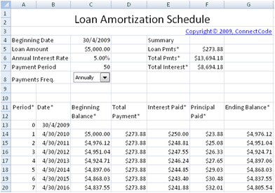
Loan Amortization Schedule with Additional Payments
The “Loan Sched-Additional Payments” worksheet allows for additional payments to be catered for each period. This is as shown in the blue color shaded field below. The loan schedule will be automatically adjusted when the additional payments are added into the spreadsheet.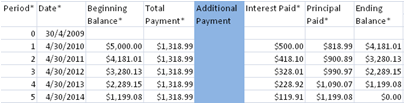
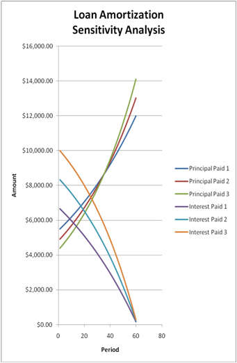
Loan Amortization Schedule with Sensitivity Analysis
This “Sensitivity Analysis” worksheet is an advance loan amortization schedule that performs sensitivity analysis over varying interests. The inputs for this worksheet are almost the same as a normal loan amortization schedule. In cells H52 to O52, you will be able to key in varying interests to perform the sensitivity analysis. Two sensitivity analysis tables on Principal Paid over varying Interests and Interest Paid over varying Interests are already generated for performing the analysis. The spreadsheet uses the Excel “What If -> Data Table” functionalities to vary the interest rates and calculating the figures in the table easily.The chart below shows the output of the Data Tables in a graphical form. It basically illustrates the amount of the loan repayments that goes into paying the principal amount and repayments that go into paying the interest over time. The different lines shows the effects of the varying interests rate.
Customizing the Loan Amortization Schedule
Supporting a longer loan amortization period
The default loan amortization schedule supports up to 127 payment schedules. However this can be easily customized to support more schedules. Simply select the last line of the loan schedule worksheet, cell A140 to G140 and copy this line further down the rows to extend the number of maximum schedules.The only other potential change is in cell F6, the Total Pmts field. By default this field is already set to the following:
=SUM(D14:D846)
This means it will already be able to sum the loan schedules up to row 846. If you have extended the loan amortization schedules to beyond row 846 in the previous step, then you can change the SUM formula above to include the additional rows. For example, if you extend the loan schedules to row 900, simply change cell F6 to:
=SUM(D14:D900)
Important fields in the spreadsheet
This section is for advance users who intend to perform advance customization or integrate the template with other financial models. It describes the key fields in the spreadsheet worth highlighting to help you understand the spreadsheet in details. It is optional if you only intend to use the spreadsheet.Loan Amortization Schedule
Loan Pmts fieldThis field is set as :
=PMT(C6/PMNTFREQ(C8),C7,-C5,0,0)
It uses Microsoft Excel PMT function to calculate the payment for a loan based on constant payments and a constant interest rate. The PMT function is defined as follow :
=PMT(rate,nper,pv,fv,type)
The parameter rate is the interest rate for the loan, nper is the number of payments and pv is the principal value. fv and type are not used. For a more complete description of this function refer to the Excel documentation.
It is important to take note how the interest is calculated and used in the PMT function. For example, if the loans repayment frequency is set to Monthly and the Annual Interest Rate is 12% then the interests rate each month will be calculated as (0.12/12) where the value 12 is calculated using the PMNTFREQ(C8) Visual Basic for Applications formula. The user defined PMNTFREQ VBA formula is included in the spreadsheet and is defined as follow.
Function PMNTFREQ(ByVal x As Integer) As Double

If (x = 1) Then
    PMNTFREQ = 1
ElseIf (x = 2) Then
    PMNTFREQ = 2
ElseIf (x = 3) Then
    PMNTFREQ = 4
ElseIf (x = 4) Then
    PMNTFREQ = 6
ElseIf (x = 5) Then
    PMNTFREQ = 12
ElseIf (x = 6) Then
    PMNTFREQ = 52.1428571429
End If

End Function
The function returns the payments frequency based on the Payments Period as shown below.
| Payments Period | Number to return |
| Annually | 1 |
| Semi-Annually | 2 |
| Quarterly | 4 |
| Bi-Monthly | 6 |
| Monthly | 12 |
| Weekly | 52.1428571429 |
Payments Freq. field
The Payments Freq. field is defined using a control. The control is set to list the following selections.
| Payments Period |
| Annually |
| Semi-Annually |
| Quarterly |
| Bi-Monthly |
| Monthly |
| Weekly |
When a selection is made, the control will return a number to cell C8. The number returned is used by the PMNTFREQ VBA function as described in the previous section.
| Payments Period | Number to return |
| Annually | 1 |
| Semi-Annually | 2 |
| Quarterly | 3 |
| Bi-Monthly | 4 |
| Monthly | 5 |
| Weekly | 6 |
Date field
The Date output field in the amortization schedule uses the AMRTDATE VBA function which is defined in the table below. The function uses the payment frequency field and the Excel DateAdd function to calculate the dates in the schedule.
Function AMRTDATE(ByRef mycell As Range,
ByVal x As Integer) As Date

If (x = 1) Then
    AMRTDATE = DateAdd("yyyy", 1, mycell.Value)
ElseIf (x = 2) Then
    AMRTDATE = DateAdd("m", 6, mycell.Value)
ElseIf (x = 3) Then
    AMRTDATE = DateAdd("m", 4, mycell.Value)
ElseIf (x = 4) Then
    AMRTDATE = DateAdd("m", 2, mycell.Value)
ElseIf (x = 5) Then
    AMRTDATE = DateAdd("m", 1, mycell.Value)
ElseIf (x = 6) Then
    AMRTDATE = DateAdd("d", 7, mycell.Value)
End If

End Function
Loan Sched-Additional Payments
Ending Balance fieldThe Loan Sched-Additional Payments worksheet is very similar to the Loan Amortization Schedule worksheet. It supports an additional field call Additional Payment and the only other change is the Ending Balance field which is now defined as below.
Ending Balance = Beginning Balance - Principal Paid - Additional Payment
Sensitivity Analysis
Sensitivity Analysis – Annual Interest Rate fieldsThe Sensitivity Analysis worksheet uses Excel Data Table to perform sensitivity analysis on the loan schedule by varying the interest rate. A data table is a range of cells that shows how changing one or two variables in your formulas can affect the results of those formulas.
The following steps are carried out to create the Data Table in this worksheet.
1. Select the range G52 to J112
2. On the Data tab, in the Data Tools group, click What-If Analysis, and then click Data Table.
3. Set the Row input cell to C6
Similar steps are use to create the second Data Table on the worksheet.
Back to Free Loan Amortization Schedule